|
||||||||||||||||||||||||||||||||||||||||||||||||||||||||||||||||||||||||||||||||||||||||||||||||||||||||||||||||||||||||||||||||||||||||||||||||||||||||||||||||||||||||||||||||||||||||||||||||||||||||||||||||||||||||||||||||||||||||||||||||||||||||||||||||||||||||||||||||||||||||||||||||||||||||||||||||||||||||||||||||||||||||||||||||||||||||||||||||||||||||||||||||||||||||||||||||||||||||||||||||||||||||||||||||||||||||||||||||
| Plant to Plant Variability in Corn Production (Agronomy Journal) | ||||||||||||||||||||||||||||||||||||||||||||||||||||||||||||||||||||||||||||||||||||||||||||||||||||||||||||||||||||||||||||||||||||||||||||||||||||||||||||||||||||||||||||||||||||||||||||||||||||||||||||||||||||||||||||||||||||||||||||||||||||||||||||||||||||||||||||||||||||||||||||||||||||||||||||||||||||||||||||||||||||||||||||||||||||||||||||||||||||||||||||||||||||||||||||||||||||||||||||||||||||||||||||||||||||||||||||||||
|
Plant-to-Plant Variability in Corn Production K.L. Martin, P.J. Hodgen, K.W. Freeman, Ricardo Melchiori, B. Arnall, R.W. Mullen, K. Desta, S.B. Phillips, W.R. Raun, J.B. Solie, M.L. Stone, Octavio Caviglia, Hailin Zhang, Agustin Bianchini, D.D. Francis, J.S. Schepers, and J. Hatfield.
Oklahoma State University, Stillwater, OK; Nacional Soil Tilth Laboratory, Ames,
IA;
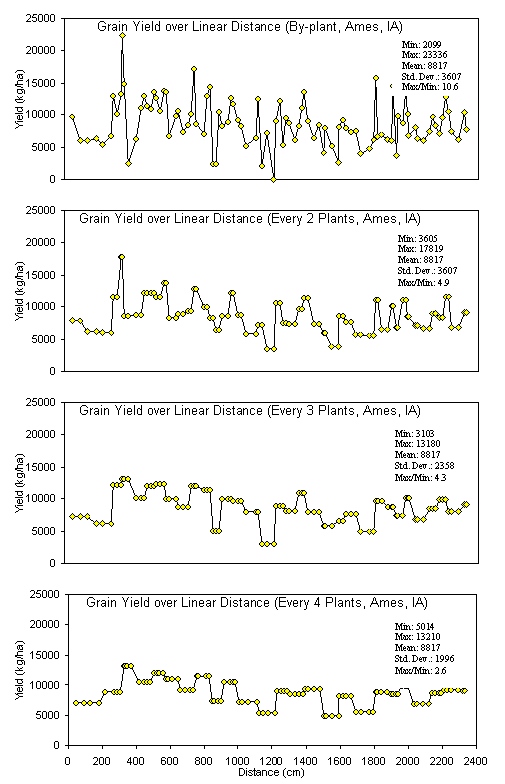
Introduction In accordance with the countries and states where data was collected from this trial, the following production statistics are provided. In 2003, world corn grain production averaged 4.5 Mg ha-1, coming from 142 million hectares. Average corn grain production in the USA, Argentina, and Mexico was 8.9, 6.4, and 2.5 Mg ha-1 from 28, 2.3, and 7.8 million hectares, respectively (http://faostat.fao.org). In Iowa, Nebraska, Ohio, Virginia, and Oklahoma, average corn production for 2003 was 9.8, 9.2, 8.7, 7.2 and 7.8 Mg ha-1 from 4.8, 3.1, 1.2, and 0.08 million hectares, respectively (http://www.usda.gov/nass/nasshome.htm). Variability in plant stands has been well known for some time. Work by Nielsen (2001) studied plant spacing variability (PSV) in 354 commercial fields of corn throughout Indiana and Ohio. This work showed that the standard deviation of plant spacing was 7.5 cm or less in only 16% of the fields. Sixty percent of the sampled fields exhibited standard deviations of plant spacing between 10 and 12.5 cm. Plant spacing variability in 24% of the fields was 15 cm or greater (up to 30 cm). Their results further noted that for every 2.54 cm increase in the standard deviation in plant-to-plant spacing, 156 kg ha-1 (2.5 bu ac-1) in grain yield were lost. The average standard deviation of plant spacing was 17.2 cm (6.8 in), resulting in an estimated 1066 kg ha-1 (17 bu ac-1) yield loss over 354 commercial fields. Nafziger et al. (1991) noted that uneven emergence of corn can occur when soils are dry at the time of planting and could lead to decreased grain yields. It is generally accepted that when adjacent plants differ by more than 2 leaf stages, the younger plant will be barren. A 2-leaf stage difference can result from delayed emergence ranging from 5-10 days and the yield loss from late emergence could be 1% for each 1 day delay (Robert L. Nielsen, Purdue University, personal communication, February 10, 2004). These staggering statistics target a two-fold problem, first the need to homogenize plant spacing and emergence, and secondly, the need to recognize differences in yield potential that clearly exist by-plant. Current thinking in precision agriculture has to some extent been driven by the technologies that specific companies have promoted and/or financed. The most notable has been combine yield-monitors. Depending on combine speed, header width, and the smoothing effect as grain moves through the combine, each sensed element represents more than 80 m2. This is disturbing because Lengnick (1997), Solie et al. (1999), and Raun et al. (1998) all found significant soil variability at distances less than 30 m apart, and in many cases, less than 1 m2. Furthermore, large differences in measured yield have been reported on a small scale (< 0.4 m2) for winter wheat (Raun et al., 2002) and by plant in corn (Raun et al., 2005). For corn, the expressed spatial variability was greatest at the V6 growth stage, and this peak in the within-row, by-plant variability was thought to be the same growth stage where treating the variability would have the greatest impact (Raun et al., 2005). Maddonni and Otegui (2004) reported that the largest difference in estimated shoot biomass between plant types took place between V7 and V13 and remained constant from V13 onwards. In this regard, Varvel et al. (1997) noted that when sufficiency indices were lower than 90% at V8, maximum yields were not achieved with in-season N fertilizer applications because early season N was below that needed for optimum growth and yield potentials had already been reduced. Therefore, if added N were needed, making the decision to apply should likely take place at or before V8. Materials and Methods By plant harvesting of corn grain yield was evaluated at 13 different sites in Argentina, Mexico, Iowa, Nebraska, Ohio, Virginia, and Oklahoma. At each location, corn rows (transects) ranging from 8.1 to 30 m in length were selected for by-plant harvesting. At most of the sites, individual plants were marked at or before the V8 growth stage to assure detection of barren, and/or lost plants at harvest (60-85 days later depending on the maturity). At the same time that plants were tagged, a tape measure was laid down at plant 1 and extended to the final plant in each row. With the tape measure in place, cumulative distances were recorded for each plant in each row. At most sites, based on the row spacing used at each location, the area occupied by each plant was calculated. This was done by assuming that each plant occupies half the distance to and from its nearest neighbor (Equation 1). Area (cm) = [(1/2) B – A] + [(1/2) C – B] *(R) (1) Where: A is the plant before the plant in question. B is the plant in question. C is the plant following the plant in question. R is the row spacing. Each ear was harvested individually from each plant and weights recorded. At those sites where actual distances between plants were not recorded, an average distance occupied per plant was determined based on row spacing and total transect or row distance and number of plants harvested per row. The plant was then weighed with the ear attached for the wet biomass weights. Once removed from the stalk, ears were dried at 66°C for 48 hours and weighed before and after shelling. The weight taken from the dry, shelled corn was the final grain weight used for yield determination. Statistical analysis included regression of average grain yield per transect on the standard deviation, coefficient of variation (CV), and yield range of by-plant grain yield over all locations. The areas where by-plant harvest data was collected were representative of a range of corn production environments around the world. Results Average transect corn grain yield plotted against standard deviation, CV, and yield range over all locations is illustrated in Figures 1, 2, and 3, respectively. Excluding the Phillips, NE transects, the standard deviation of by-plant corn grain yields increased with increasing yield level (Figure 1). This is consistent with several sources noting that the standard deviation of yields increases with increasing yield level (Taylor et al., 1999, Dobermann et al., 2003). The CV of by-plant yields was negatively correlated with mean grain yield across the range of experiments studied (Figure 2). The yield range (maximum yield observed in each transect minus the minimum yield observed) increased with average corn grain yields (Figure 3), excluding the Phillips, NE transects. Average grain yields across all regions ranged from 4268 to 14383 kg ha-1, with an average of 8495 kg ha-1 (135 bu ac-1), right at the USA average and above that for Argentina and Mexico. The average differences in actual yield that could be expected, plant-to-plant, ranged from 1724 to 4367 kg ha-1 and averaged 2765 kg ha-1 (44.1 bu ac-1) (Table 3). It is important to note that at those sites where the average yields were the highest (Phillips, NE, and Argentina), average plant to plant differences in yields were 2926 kg ha-1 (47 bu ac-1) and 4211 kg ha-1 (67 bu ac-1). Although a trend for decreased CVs at the higher yield levels was observed (Figure 2), the average plant-to-plant yield differences that would be encountered at both these high yielding sites exceeded the average over all locations where yields were much lower. Discussion Inherent and acquired variability in the production system encompasses all of the factors that cause plant-to-plant variability. These results suggest that the combined components of variability (planting depth, tillage, compaction, moisture, etc) create the underlying plant-to-plant variability, and that was consistent across production fields, and nearly independent of yield level. Even though CVs were lower for the higher yielding sites, the plant-to-plant variation in actual yield levels in kg ha-1 was much greater. If plant-to-plant variation in yield was known to be 2765 kg ha-1 (44.1 bu ac-1), would we not want to recognize these differences and treat them? That the plant-to-plant differences in actual grain yield did not decrease with increasing yield level suggests that plant-to-plant yield levels need to be recognized in all environments. If it is feasible to recognize 2765 kg ha-1 plant-to-plant yield differences when average yields are 4300 kg ha-1, it will be feasible to recognize them when average yields are 14000 kg ha-1. The current N rate recommendation strategy in Nebraska = 35+(1.2*EY)-(8*NO3-N)-(0.14*EY*OM), where EY is expected yield in bu ac-1, NO3-N is the ppm in the preplant soil test and OM is the % organic matter (Richard Ferguson, University of Nebraska, personal communication, August 2004). For a soil with 2.0% OM and 10 ppm NO3-N, the N rate recommendation in lb/ac for a 230 bu ac-1 yield goal will be 167 lb N ac-1 or 187 kg N ha-1. If, for example, the average plant to plant differences in yield were 43 bu ac-1, N demand should change (on average, 1.2*43) by 51.6 lb ac-1 or 57.7 kg N ha-1. This represents an average of 1/3 the total (187 kg N ha-1) and that changes by this amount or more from plant to plant. This can hardly be viewed as a precise fertilizer N strategy in light of the large differences in plant-to-plant yields. Based on the yield goal, this means that the average N rate will be off by more than 31% for each plant. Variable rate N technologies are already available that can sense and fertilize each corn plant on-the-go, altering rates in intervals of 10 kg ha-1 (http://www.nue.okstate.edu). Considering the incredibly large differences noted in these studies and that were encountered at all yield levels, it will be important to re-focus on this by-plant variability in corn grain yields if increased NUE and profitability are to be achieved. Even if the errors in predicting actual yield were off by 100%, this error is quite small next to the 11.1X (1110%) average difference in corn grain yields found in less than 30 m of row over all sites (Table 3). Work by Taylor et al., (1999) showed that standard deviations about yield means increased as mean yields increased in 220 fertilizer, weed management, and tillage trials. Excluding the Phillips, NE data, this is precisely what was encountered in these trials. Also, the Taylor et al., (1999) work reported a decrease in yield CV when mean yields increased. However, unlike the Taylor et al., (1999) work, which focused on plot data, we report on the standard deviations associated with by-plant differences in measured grain yield, and that realistically were expected to be different. The average maximum/minimum range observed was 11.1X (45 transects ranging from 8 to 39 m of row). This comes from experiments with an average yield of 8495 kg ha-1 well above the World average of 4500 kg ha-1 reported for corn grain yield in 2003. Furthermore, the data collected at specific sites within each location (Argentina, Mexico, Iowa, Nebraska, Ohio, and Oklahoma) had yields equal to or exceeding each specific region’s average. Dobermann et al. (2003) reported corn grain yields from 4x4m grids determined from yield monitor data from 1996 to 2001. In this work, the maximum/minimum yields observed in the entire field exceeded 20X. For the data in Figure 4, grain yields were determined based on actual measured distances between plants and the area each occupied as reported in Materials and Methods, and that resulted in 10.6X differences in corn grain yield over 15m of row. However, it is important to note that when by-plant grain yields were computed based on a fixed area (average distance between plants, 23.5 cm, over the entire row), a 12.5X difference in yield differences was observed at the Ames, IA site (data not reported). At all sites, large differences in corn grain yield were observed over short distances whether or not grain yields were computed based on actual measured distances or an average (fixed) distance between plants. If it were not possible to recognize each plant individually using sensors as has been published, it would be considered important to evaluate different scales. Subsequently, by-plant grain yields were combined into averages over 2, 3, and 4 plants in 15 m of row from the Ames, IA location (Figure 4). It was clear that the big differences in yield were discernable at the by-plant level. However, 4.9, 4.3, and 2.6X differences were detected within 15 m of row when averaged over 2, 3, and 4 plants, respectively (Figure 4). At this site, the average differences in yield (standard deviation) were 3607, 2678, 2358, and 1996 kg ha-1, when yields were averaged over 1, 2, 3, and 4 plants. The telling statistic here is that even when averaged over every 4 plants, this scale resulted in average differences between 4-plant clusters that exceeded 1900 kg ha-1 (30 bu ac-1). In addition, when evaluating every 4-plant cluster in 15 m of row, the range in yields was 5014 to 13210 kg ha-1 (difference of 8196 kg ha-1 or 131 bu ac-1). Considering that predicting yield mid-season has been successfully demonstrated in wheat (Raun et al., 2002) and corn (Raun et al., 2005), it was encouraging to find the large differences in actual yield within 15 m of row, regardless of the scale evaluated (average of 1, 2, 3, or 4 plants). At this site, mid-season prediction of corn grain yields (same 4 plant clusters) was quite good using NDVI collected at the V8 growth stage (Figure 5). The average yield difference of 1996 kg ha-1 between each 4-plant cluster was greater than the precision at which final grain yields could be predicted mid-season using NDVI (precision of ± 1565? kg ha-1). Because the error in predicting final grain yield using mid-season sensor readings was smaller than the average differences in harvested grain yield between every 4-plant cluster, management based on predicted yields at this scale can be expected to result in improved precision and use efficiency. Considering the above data from Iowa (4 plant clusters average length of 94cm, in 76 cm rows), it is important to extrapolate this to a by-row scenario. If N deficiencies are present, it is common for them to be visibly discernable from one row to the next. This being the case in production environments, it is logical that the scale at which N should be applied should be no greater than the distance between rows (commonly 76 cm). Furthermore, it is not surprising to find the exact same phenomenon (visible differences in growth) when evaluating N response in linear rows (with and without N). The same minimum resolution of 76 cm (where N effects are discernable) should hold true whether it is left and right or front and back, which is in fact the case. So what is the cause of the extensive variability in by-plant corn grain yield seen at all sites included in this study? Delayed and uneven emergence can be caused by variable depth of planting, double seed drops, wheel compaction, seed geometry within the furrow, surface crusting, random soil clods, soil texture differences, variable distance between seeds, variable soil compaction around the seed, insect damage, moisture availability, variable surface residue, variable seed furrow closure, and/or many other factors that influence non-uniformity of plants. All of the above take place and can impact the uneven stands prior to the time that irrigation takes place whether using surface/furrow or center pivot systems. Unless there is severe drought at planting, the first irrigation seldom takes place before V4. In light of the many factors known to influence emergence, extensive within row variability in corn grain yield should be expected, and that was without question the norm in the trials evaluated here. In all trials, common hybrids were employed for each respective region. Each row was inspected early in the season (excluding the Phillips, NE location) for volunteer corn and these plants were removed. Some of the variability may have been due-to the presence of volunteer corn plants that were not discernable from the others, but this was considered to be small. This was especially true in the Oklahoma, Argentina, and Mexico where corn was not the previous crop, thus limiting any potential variability that would have been due to volunteer corn. The range of average yields (2700 to 16100 kg/ha) included in this study was representative of a wide array of production environments (Figures 1-3). Some of these sites were irrigated, while others relied on natural precipitation. One of the sources of plant-to-plant variability could be competition for soil moisture, especially at the lower yield levels. However, this would be an unlikely source of plant-to-plant variability at the higher yield levels where moisture was not limiting (>12000 kg/ha), unless soil texture differences were expected at the by-plant level. Similarly, the extensive plant to-plant differences in grain yield within 8 to 30 m of row were unlikely due to plant-to-plant differences in N availability at the higher yield levels where N was not limiting. Because standard deviations increased with increasing yield level, moisture and N availability were unlikely sources of the increased variability (Figure 1). However, it remains important from an N management perspective to recognize that this kind of within row variability in grain yield exists. Because N deficiencies can be seen from one row to the next (generally 76cm), fertilizing at this same scale based on yield potential, should deliver N where it is needed and at the scale where incredibly large differences in yield potential exist within rows. Because large differences in yield potential exist at resolutions of <4 plants (Figure 4) that occupied a linear distance of 70 cm, and it is known the visual differences are easily recognizable by-row (normally 76 cm wide), applications at this same scale can deliver N fertilizer based on need. Maddonni and Otegui (2004) noted that increased interplant competition in corn hybrids enhanced the appearance of plants with different competitive abilities. Thus at higher populations, plant-to-plant variation can also be expected. They noted that the onset of interplant competition started very early during the growing cycle, and that estimated plant biomass between stand densities were detected as early as V6. Furthermore, they reported that plant population and row spacing treatments did not modify the onset of the hierarchical growth among plants. Because yield potential can be predicted early in the season, nutrient management decisions can be made based on predicted yield potential and nutrient removal (at a specific yield potential), especially when considering that the average differences were 11.1X in 8-30 m of row (Table 3). Even though there are clearly errors associated with predicting yield at early growth stages (V8, Figure 5), these errors in yield prediction are dwarfed in comparison to the 11.8X average differences in by-plant yield within row. Thus, as was noted earlier, even if yield prediction were off by 100%, it is an incredibly small error next to the 1110% differences in actual yield. Recognizing and treating the differences in yield potential based on predicted amounts of nutrient removal will lead to a vastly improved mid-season N management, provided that by-plant yield prediction is possible.
References Dobermann, A., J.L. Ping, V.I. Adamchuk, G.C. Simbahan, and R.B. Ferguson. 2003. Classification of crop yield variability in irrigated production fields. Agron. J. 95:1105-1120. Lengnick, 1997. Spatial variation of early season nitrogen availability indicators in corn. Commun. Soil Sci. Plant Anal. 28:1721-1736. Mallarino, A.P., E.S. Oyarzabal, and P.N. Hinz. 1999. Interpreting within-field relationships between crop yields and soil and plant variables using factor analysis. Precision Agric. 1:15-25. Maddonni, G.A., and M.E. Otegui. 2004. Intra-specific competition in maize:early establishment of hierarchies among plants affects final kernel set. Field Crops Res: 85:1-13. Nafziger, E.D., P.R. Carter, and E.E. Graham. 1991. Response of corn to uneven emergence. Crop Sci. 31:811-815. Nielsen, R.L. 2001. Stand establishment variability in corn. Purdue University, Dept. of Agronomy Publication #AGRY-91-01. Porter, P.M., J.G. Lauer, D.R. Huggers, E.S. Oplinger, and R.K. Crookston. 1998. Assessing spatial and temporal variability of corn and soybean yields. J. Prod. Agric. 11:359-363. Raun, W.R., J.B. Solie, G.V Johnson, M.L. Stone, R.W. Whitney, H.L. Lees, H. Sembiring and S.B. Phillips. 1998. Micro-variability in soil test, plant nutrient, and yield parameters in bermudagrass. Soil Sci. Soc. Am. J. 62:683-690. Raun, W.R., J.B. Solie, M.L. Stone, K.L. Martin, K.W. Freeman, R.W. Mullen, H. Zhang J.S. Schepers, and G.V. Johnson. 2004a. Optical sensor based algorithm for crop nitrogen fertilization. Commun. Soil Sci. Plant Anal. (in press). Raun, W.R., J.B. Solie, K.L. Martin, K.W. Freeman, M.L. Stone, K.L. Martin, G.V. Johnson, and R.W. Mullen. 2005. Growth stage, development, and spatial variability in corn evaluated using optical sensor readings. J. Plant Nutr. 28:173-182. Raun, W.R., J.B. Solie, G.V. Johnson, M.L. Stone, R.W. Mullen, K.W. Freeman W.E. Thomason, and E.V. Lukina. 2002. Improving nitrogen use efficiency in cereal grain production with optical sensing and variable rate application. Agron. J. 94:815-820. Sadler, E.J., W.J. Busscher, P.J. Bauer, and D.L. Karlen. 1998. Spatial scale requirements for precision farming: a case study in the southeastern USA. Agron. J. 90:191-197. Schmidt, J.P., A.J. DeJoia, R.B. Ferguson, R.K. Taylor, R.K. Young, and J.L. Havlin. 2002. Corn yield response to nitrogen at multiple in-field locations. Agron. J. 94:798-806. Solie, J.B., W.R. Raun and M.L. Stone. 1999. Submeter spatial variability of selected soil and bermudagrass production variables. Soil Sci. Soc. Am. J. 63:1724-1733. Solie, J.B., W.R. Raun, R.W. Whitney, M.L. Stone and J.D. Ringer. 1996. Optical sensor based field element size and sensing strategy for nitrogen application. Trans. ASAE 39(6):1983-1992. Stone, M.L., J.B. Solie, W.R. Raun, R.W. Whitney, S.L.
Taylor and J.D. Ringer. 1996. Use of spectral radiance for correcting in-season
fertilizer nitrogen deficiencies in winter wheat. Trans. ASAE 39(5):1623-1631. Varvel, G.E., J.S. Schepers, and D.D. Francis. 1997. Ability for in-season correction of nitrogen in corn using chlorophyll meters. Soil Sci. Soc. Am. J. 61:1233-1239. |
||||||||||||||||||||||||||||||||||||||||||||||||||||||||||||||||||||||||||||||||||||||||||||||||||||||||||||||||||||||||||||||||||||||||||||||||||||||||||||||||||||||||||||||||||||||||||||||||||||||||||||||||||||||||||||||||||||||||||||||||||||||||||||||||||||||||||||||||||||||||||||||||||||||||||||||||||||||||||||||||||||||||||||||||||||||||||||||||||||||||||||||||||||||||||||||||||||||||||||||||||||||||||||||||||||||||||||||||
 Figure 1. Average corn grain yield plotted against the standard deviation of by-plant yield over 43 transects in Argentina, Mexico, Iowa, Nebraska, Ohio, and Oklahoma. |
||||||||||||||||||||||||||||||||||||||||||||||||||||||||||||||||||||||||||||||||||||||||||||||||||||||||||||||||||||||||||||||||||||||||||||||||||||||||||||||||||||||||||||||||||||||||||||||||||||||||||||||||||||||||||||||||||||||||||||||||||||||||||||||||||||||||||||||||||||||||||||||||||||||||||||||||||||||||||||||||||||||||||||||||||||||||||||||||||||||||||||||||||||||||||||||||||||||||||||||||||||||||||||||||||||||||||||||||
 Figure 2. Average corn grain yield plotted against the coefficient of variation from by-plant yield over 43 transects in Argentina, Mexico, Iowa, Nebraska, Ohio, and Oklahoma.
|
||||||||||||||||||||||||||||||||||||||||||||||||||||||||||||||||||||||||||||||||||||||||||||||||||||||||||||||||||||||||||||||||||||||||||||||||||||||||||||||||||||||||||||||||||||||||||||||||||||||||||||||||||||||||||||||||||||||||||||||||||||||||||||||||||||||||||||||||||||||||||||||||||||||||||||||||||||||||||||||||||||||||||||||||||||||||||||||||||||||||||||||||||||||||||||||||||||||||||||||||||||||||||||||||||||||||||||||||
|
Figure 3. Average corn grain yield plotted against the by-plant yield range (max minus min) in 43 transects ranging from 10.5 to 30m in length, in Argentina, Mexico, Iowa, Nebraska, Ohio, and Oklahoma.
|
||||||||||||||||||||||||||||||||||||||||||||||||||||||||||||||||||||||||||||||||||||||||||||||||||||||||||||||||||||||||||||||||||||||||||||||||||||||||||||||||||||||||||||||||||||||||||||||||||||||||||||||||||||||||||||||||||||||||||||||||||||||||||||||||||||||||||||||||||||||||||||||||||||||||||||||||||||||||||||||||||||||||||||||||||||||||||||||||||||||||||||||||||||||||||||||||||||||||||||||||||||||||||||||||||||||||||||||||
| Figure 4. Average corn grain yields plotted by plant, every 2 plants, every 3 plants and every 4 plants, Ames, IA 2004. | ||||||||||||||||||||||||||||||||||||||||||||||||||||||||||||||||||||||||||||||||||||||||||||||||||||||||||||||||||||||||||||||||||||||||||||||||||||||||||||||||||||||||||||||||||||||||||||||||||||||||||||||||||||||||||||||||||||||||||||||||||||||||||||||||||||||||||||||||||||||||||||||||||||||||||||||||||||||||||||||||||||||||||||||||||||||||||||||||||||||||||||||||||||||||||||||||||||||||||||||||||||||||||||||||||||||||||||||||
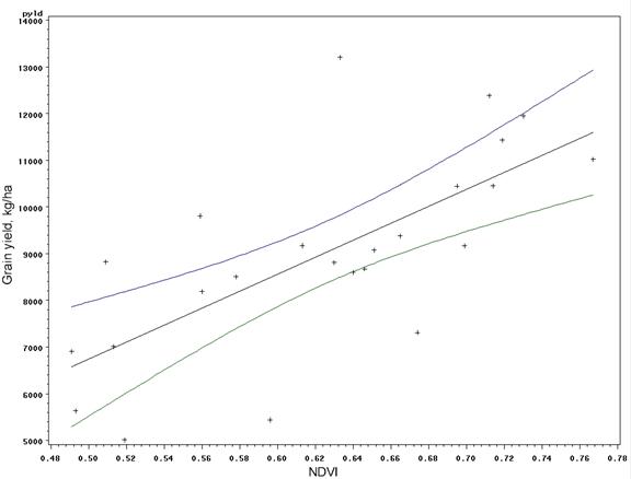 Yield =
-2348 + 18181(NDVI) Figure 5. NDVI versus corn grain yield determined for every 4 plants using linear regression and associated 95% confidence intervals, east row, Ames IA, 2004.
|
||||||||||||||||||||||||||||||||||||||||||||||||||||||||||||||||||||||||||||||||||||||||||||||||||||||||||||||||||||||||||||||||||||||||||||||||||||||||||||||||||||||||||||||||||||||||||||||||||||||||||||||||||||||||||||||||||||||||||||||||||||||||||||||||||||||||||||||||||||||||||||||||||||||||||||||||||||||||||||||||||||||||||||||||||||||||||||||||||||||||||||||||||||||||||||||||||||||||||||||||||||||||||||||||||||||||||||||||
| OTHER LINKS | ||||||||||||||||||||||||||||||||||||||||||||||||||||||||||||||||||||||||||||||||||||||||||||||||||||||||||||||||||||||||||||||||||||||||||||||||||||||||||||||||||||||||||||||||||||||||||||||||||||||||||||||||||||||||||||||||||||||||||||||||||||||||||||||||||||||||||||||||||||||||||||||||||||||||||||||||||||||||||||||||||||||||||||||||||||||||||||||||||||||||||||||||||||||||||||||||||||||||||||||||||||||||||||||||||||||||||||||||
| Estimating Corn Yield Losses from Uneven Plant Spacing (Carlson, Doerge, Clay) | ||||||||||||||||||||||||||||||||||||||||||||||||||||||||||||||||||||||||||||||||||||||||||||||||||||||||||||||||||||||||||||||||||||||||||||||||||||||||||||||||||||||||||||||||||||||||||||||||||||||||||||||||||||||||||||||||||||||||||||||||||||||||||||||||||||||||||||||||||||||||||||||||||||||||||||||||||||||||||||||||||||||||||||||||||||||||||||||||||||||||||||||||||||||||||||||||||||||||||||||||||||||||||||||||||||||||||||||||
|
By-plant variability in corn grain yield (45 transects)
Causes
of By-Plant Variability in Corn Production Systems |
||||||||||||||||||||||||||||||||||||||||||||||||||||||||||||||||||||||||||||||||||||||||||||||||||||||||||||||||||||||||||||||||||||||||||||||||||||||||||||||||||||||||||||||||||||||||||||||||||||||||||||||||||||||||||||||||||||||||||||||||||||||||||||||||||||||||||||||||||||||||||||||||||||||||||||||||||||||||||||||||||||||||||||||||||||||||||||||||||||||||||||||||||||||||||||||||||||||||||||||||||||||||||||||||||||||||||||||||
|
By-plant variability in corn grain yield (45 transects) (Included in
this study are data from Argentina, Mexico, Nebraska, Iowa, Ohio, Virginia,
Oklahoma)
|
||||||||||||||||||||||||||||||||||||||||||||||||||||||||||||||||||||||||||||||||||||||||||||||||||||||||||||||||||||||||||||||||||||||||||||||||||||||||||||||||||||||||||||||||||||||||||||||||||||||||||||||||||||||||||||||||||||||||||||||||||||||||||||||||||||||||||||||||||||||||||||||||||||||||||||||||||||||||||||||||||||||||||||||||||||||||||||||||||||||||||||||||||||||||||||||||||||||||||||||||||||||||||||||||||||||||||||||||
Return to
 |
||||||||||||||||||||||||||||||||||||||||||||||||||||||||||||||||||||||||||||||||||||||||||||||||||||||||||||||||||||||||||||||||||||||||||||||||||||||||||||||||||||||||||||||||||||||||||||||||||||||||||||||||||||||||||||||||||||||||||||||||||||||||||||||||||||||||||||||||||||||||||||||||||||||||||||||||||||||||||||||||||||||||||||||||||||||||||||||||||||||||||||||||||||||||||||||||||||||||||||||||||||||||||||||||||||||||||||||||