
Plant-to-Plant
Variability in Corn Production
Oklahoma State University; USDA-ARS, Lincoln, NE; Stillwater, OK; National Soil Tilth Laboratory, Ames, IA; Asociacion Argentina de Productores en Siembra Directa, Rosario, Argentina; Ohio State University, Virginia Polytechnic Institute; Instituto Nacional de Tecnologia Agropecuaria (INTA), Parana, Argentina
(Agron. J. 2005, 97:1603-1611) (pdf)
Abstract
Corn grain yields are known to vary from plant to plant, but the extent of
this variability across a range of environments has not been evaluated. This
study was initiated to evaluate by-plant corn grain yield variability over a
range of production environments and to establish the relationships between mean
grain yield, standard deviation, coefficient of variation, and yield range. A
total of forty-six 8 to 30-m corn transects were harvested by plant in
Argentina, Mexico, Iowa, Nebraska, Ohio, Virginia, and Oklahoma from 2002 to
2004. By-plant corn grain yields were determined and the average individual
plant yields were calculated. Over all sites in all countries and states,
plant-to-plant variation in corn grain yield averaged 2765 kg ha-1 (44.1 bu
ac-1). At the sites with the highest average corn grain yield (11478 and 14383
kg ha-1, Parana Argentina, and Phillips, NE), average plant-to-plant variation
in yield was 4211 kg ha-1 (67 bu ac-1) and 2926 kg ha-1 (47 bu ac-1),
respectively. As average grain yields increased, so did the standard deviation
of the yields obtained within each row. Furthermore, the yield range (maximum
corn grain yield minus the minimum corn grain yield per row) was found to
increase with increasing yield level. This work shows that regardless of yield
level, plant-to-plant variability in corn grain yield can be expected and
averaged more than 2765 kg ha-1 over sites and years. Averaging yield over
distances >0.5 m removed the extreme by-plant variability, thus, the scale for
sensing and treating other factors affecting yield should be less than 0.5 m.
Production methods that homogenize plant stands and emergence, should decrease
plant-to-plant variation and will likely lead to increased yields.
Introduction
In accordance with the countries and states where data were collected for this paper, the following production statistics are provided. In 2003, world corn grain production averaged 4.5 Mg ha-1, coming from 142 million hectares. Average corn grain yields in the USA, Argentina, and Mexico was 8.9, 6.4, and 2.5 Mg ha-1 from 28, 2.3, and 7.8 million hectares, respectively (http://faostat.fao.org). In Iowa, Nebraska, Ohio, Virginia, and Oklahoma, average corn grain yield for 2003 was 9.8, 9.2, 8.7, 7.2 and 7.8 Mg ha-1 from 4.8, 3.1, 1.2, 0.13, and 0.08 million hectares, respectively (http://www.usda.gov/nass/nasshome.htm).
Variability in plant stands is well documented. Nielsen (2001) studied plant spacing variability (PSV) in 354 commercial fields of corn throughout Indiana and Ohio. This work showed that the standard deviation of plant spacing was 7.5 cm or less in only 16% of the fields. Sixty percent of the sampled fields exhibited standard deviations of plant spacing between 10 and 12.5 cm. Plant spacing standard deviations in 24% of the fields was 15 cm or greater (up to 30 cm). Their results showed that for every 2.54 cm increase in the standard deviation in plant-to-plant spacing, 156 kg ha-1 (2.5 bu ac-1) in grain yield were lost. The average standard deviation of plant spacing was 17.2 cm (6.8 in), resulting in an estimated 1066 kg ha-1 (17 bu ac-1) yield loss over 354 commercial fields. Nafziger et al. (1991) noted that uneven emergence of corn can occur when soils are dry at the time of planting and could lead to decreased grain yields. It is generally accepted that when adjacent plants differ by more than 2 leaf stages, the younger plant will be barren. A 2-leaf stage difference can result from delayed emergence ranging from 5-10 days, which cause a 1% yield loss for each 1-day delay (Robert L. Nielsen, Purdue University, personal communication, February 10, 2004). These statistics identify a two-fold problem, first the need to homogenize plant spacing and emergence, and secondly, the need to recognize differences in yield potential that clearly exist by-plant.
Current thinking in precision agriculture has to some extent been driven by the technologies that specific companies have promoted and/or financed. The most notable has been combine yield-monitors. Depending on combine speed, header width, and the smoothing effect as grain moves through the combine, each sensed element represents more than 48 m2 (width of swath times the distance traveled in 2 to 4 s). However, Lengnick (1997), Solie et al. (1999), and Raun et al. (1998) found significant soil variability at distances less than 30 m apart, and in many cases, less than 1 m. Furthermore, large differences in measured yield have been reported on a small scale (< 0.4 m2) for winter wheat (Raun et al., 2002) and by plant in corn (Raun et al., 2005). For corn, the expressed spatial variability was greatest at the V6 growth stage. This peak in the within-row variability was thought to occur at the same growth stage where treating the variability would have the greatest impact (Raun et al., 2005). Maddonni and Otegui (2004) reported that the greatest difference in estimated shoot biomass between plant types occurred between V7 and V13 and remained constant from V13 onwards. Vega and Sadras (2003) found a strong inequality in reproductive output within high populations of maize indicating an apparent breakage of reproductive allometry.
Varvel et al. (1997) noted that when sufficiency indices (determined with a SPAD meter) were lower than 90% at V8, maximum yields were not achieved with in-season N fertilizer applications because early season available N was below that needed for optimum growth and yield potentials had already been reduced. Therefore, if added N were needed, making the decision to apply should likely take place at or before V8.
Fundamental field element size is the area where maximum relatedness exists between adjacent elements. Treatment at scales larger than the fundamental field element size compromises the effectiveness since independent variation of nutrient levels exists within a single treatment level. Treatment at scales less than the fundamental field element size is pointless, as nutrient levels within this scale are related. When N decisions are at 1 m2 resolution, the variability present can be detected (e.g., NDVI) and treated accordingly with foliar N (Solie et al., 1996; Stone et al., 1996), thus increasing NUE. Taylor et al. (1999) reported that smaller plot sizes employed in variety trials reduced the variability encountered in estimating the mean yield. This was consistent with the resolution where detectable differences in soil test parameters exist that should be treated independently.
Porter et al. (1998) observed that temporal yield variability was approximately 3 times greater for soybeans and 4 times greater for corn than spatial variability among plots. They also reported that producers should not change management practices (as a function of yield maps) unless the differences were shown to be consistent over years. Mallarino et al., (1999) employed grid sampling and factor analysis to investigate the relationship between several site variables (soil tests, plant population, weed control, etc.) and corn grain yields in 5 producer fields. They reported that some of the variables collected were correlated with grain yields, but that the relationships changed between fields. When collecting corn grain yield data from 24, 4.6x3.0 m sub-plots within a larger farmer field, Schmidt et al. (2002) showed that yields ranged from 4.7 to 9.5 Mg ha-1. It is important to note that this large range in yield was from plots that did not receive any fertilizer N. They also noted that variable N application is needed to achieve maximum grain yield and improved N management over different locations in the same field. Sadler et al. (1998) noted that Coastal Plain soils required study at finer resolutions than the >100 m grids commonly used in precision farming.
The objectives of this study were to evaluate by-plant corn grain yield
variability over a range of production environments and to determine the
relationships among mean grain yield, standard deviation of yield, coefficient
of variation of yield, and yield range.
Materials and Methods
By-plant harvested corn grain yields from 13 different sites in Argentina, Mexico, Iowa, Nebraska, Ohio, Virginia, and Oklahoma were evaluated to determine relationships among by-plant and averaged yield and ranges, standard deviations and coefficients of variation of yields. At each location, corn rows (transects) ranging from 8 to 30 m in length were selected for by-plant harvesting. At most of the sites, individual plants were marked at or before the V8 growth stage to ensure detection of barren, and/or lost plants at harvest (60-85 days later depending on the maturity). At the same time that plants were tagged, a tape measure was extended the length of the row and cumulative distances were recorded for each plant.
At most sites, based on the row spacing used at each location, the area occupied by each plant was calculated. This was done by assuming that each plant occupied half the distance to and from its nearest neighbor (Equation 1).
![]()
[1]
Where:
Ai is the area occupied by the ith plant
Di-1,di,di+1 are the distances to the i-1, i, and i+1 plants
R is the row spacing
Each ear was harvested individually from each plant and weight recorded. When more than one ear per plant was present, total weight was recorded on a by-plant basis. At those sites where actual distances between plants were not recorded, an average distance occupied per plant was determined based on row spacing and total transect or row distance and number of plants harvested per row. Once removed from the stalk, ears were dried at 66C for 48 hours and weighed before and after shelling. The weight taken from the dry, shelled corn was the final grain weight used for yield determination. All locations sampled, number of transects, planting date, harvest date, row spacing, plant population, hybrid and maturity are reported in Table 1. Location, soil series, texture, and transect length are included in Table 2.
Statistical analysis included regression of average grain yield per transect
on the standard deviation, coefficient of variation (CV), and yield range of
by-plant grain yield over all locations. The areas where by-plant harvest data
were collected were representative of a range of corn production environments
around the world. The previous crop and tillage practice employed at each site
are reported in Table 2.
Results
Average transect corn grain yield plotted against standard deviation, CV, and yield range over all locations is illustrated in Figures 1, 2, and 3, respectively. Prediction equations reported and plotted on Figures 1-3, go beyond the extent for which data were recorded, but that were useful when considering theoretical limits. The standard deviation of by-plant corn grain yield increased with increasing yield level up to 13000 kg/ha, and then tended to decrease (Figure 1). This is consistent with several sources reporting that the standard deviation of yields increases with increasing yield level (Taylor et al., 1999; Dobermann et al., 2003). The CV of by-plant yields was negatively correlated with mean grain yield across the range of experiments studied (Figure 2). Even though CVs were lower for the higher yielding sites, the actual plant-to-plant variation in grain yield (kg/ha) was greater when compared to sites with lower average yields. The yield range (maximum yield observed in each transect minus the minimum yield observed) increased with average corn grain yields and then tended to decrease for the higher yielding sites (Figure 3).
Average grain yield across all regions ranged from 4268 to 14383 kg ha-1,
with an average of 8495 kg ha-1 (135 bu ac-1), close to the USA average and
above that for Argentina and Mexico (Table 3). The average differences in
measured yield plant-to-plant ranged from 1724 to 4367 kg ha-1 (excluding barren
plants) and averaged 2765 kg ha-1 (44.1 bu ac-1) (Table 3). At those sites where
the average yields were the highest (Phillips, NE, and Argentina), the standard
deviations about the yield mean were 2926 kg ha-1 (47 bu ac-1) and 4211 kg ha-1
(67 bu ac-1), respectively. Although a trend for decreased CVs at the higher
yield levels was observed (Figure 2), the average plant-to-plant yield
differences that would be encountered at both these high yielding sites exceeded
the average over all locations where yields were much lower.
Discussion
The sites reported in this paper were planted and treated using normal
practices in each region. No extraordinary steps were taken to minimize
cultural, nutrient, or environmental factors that would keep the corn hybrids
from achieving their genetic yield potential. To achieve the theoretical maximum
genetic yield potential, stands must be optimum, plant spacing must be exact,
seed must be planted at ideal and uniform depth, all nutrients must be
non-limiting, soil types must be ideal for the cultivar, and moisture,
temperature, and all other environmental factors must be ideal during the entire
growing season. All plants must emerge within one day. All plants must set at
least one ear of corn and the ear must completely fill. Under these conditions,
the range of yield and standard deviation of yield should theoretically approach
zero.
Causes for the Large Differences in By-Plant Corn Grain Yields
So what is the cause of the extensive variability in by-plant corn grain yield seen at all sites included in this study? Delayed and uneven emergence can be caused by variable depth of planting, double seed drops, wheel compaction, location of the seed within the furrow, surface crusting, random soil clods, soil texture differences, variable distance between seeds, variable soil compaction around the seed, insect damage, moisture availability, variable surface residue, variable seed furrow closure, and/or many other factors that influence non-uniformity of plants. All of the above take place and can impact the uneven stands prior to the time that irrigation takes place whether using surface/furrow or center pivot systems. Unless there is severe drought at planting, the first irrigation seldom takes place before V4. In light of the many factors known to influence emergence, within row variability in corn grain yield should be expected, and that was without question the norm in the trials evaluated here. In all trials, common hybrids were employed for each respective region. Each row was inspected early in the season (excluding the Phillips, NE location) for volunteer corn and these plants were removed. Some of the variability may have been due-to the presence of volunteer corn plants that were not discernable from the others, but this was considered to be small. This was especially true in Virginia, Argentina, Mexico, and some sites in Oklahoma where corn was not the previous crop (Table 2).
The range of average yields (2700 to 16100 kg ha-1) included in this study was representative of a wide array of production environments (Figures 1-3). Some of these sites were irrigated, while others relied on natural precipitation. One of the sources of plant-to-plant variability could be competition for soil moisture, especially in dryland fields. However, this would be an unlikely source of plant-to-plant variability at the higher yield levels where moisture was not limiting (>13000 kg ha-1), unless soil texture differences were expected at the by-plant level. Similarly, the extensive plant to-plant differences in grain yield within 8 to 30 m of row were unlikely due to plant-to-plant differences in N availability at the higher yield levels where N was not limiting. Because standard deviation in grain yield increased with increasing yield level, moisture and N availability were unlikely sources of the increased variability (Figure 1).
Maddonni and Otegui (2004) noted that increased interplant competition in
corn hybrids enhanced the appearance of plants with different competitive
abilities. Thus at higher populations, plant-to-plant variation can also be
expected. They noted that the onset of interplant competition started very early
during the growing cycle, and that differences in estimated plant biomass
between stand densities were detected as early as V6. Furthermore, they reported
that plant population and row spacing treatments alone did not modify the onset
of the hierarchical growth among plants.
Expression of Variability
Theoretically, the upper yield boundary of regression curves fitted for the data reported must approach zero at the genetic yield potential. Similarly, both the range and standard deviation of yield should be small near zero-yield to satisfy results reported by Taylor et al., (1999), and Dobermann et al., (2003).
Seed suppliers do not normally publish genetic yield potential data (Figures 1-3). However, the National Corn Growers Association Corn Yield Contest results (www.NCGA.com) can serve as a surrogate for these data. In order to achieve maximum yields, contest participants attempt to manage all factors under their control to minimize reduction in corn yield from the cultivars genetic yield potential. The highest first place yields for all classes from 2002, 2003, and 2004 ranged from 19,000 to 22,000 kg ha-1. One can infer that these yields approached the genetic yield potential of the corn cultivars, and by-plant yield variability would be low.
Nonlinear equations were fitted to the data using Table Curve 2D (2000). The
equations with the highest R2, which conformed to the upper and lower boundary
conditions, were selected. In all cases, a partial cubic polynomial met these
requirements. Examination of Figures 1 through 3 yielded the following
additional observations on the relationship of average corn yield to CV, range,
and standard deviation. The range and standard deviation curves peaked near
13000 kg ha-1 and declined at higher yields. However, most of that decline
occurred at yields greater than 15000 kg ha-1. The corn by-plant yield
coefficient of variation was nearly constant for yields under 10000 kg ha-1 and
declined moderately to 15000 kg ha-1. Average field scale corn yields in all
areas reported in this paper were generally much lower than 15000 kg ha-1.
Clearly, by-plant corn yield variability is large within the yield ranges
achieved by producers, as indicated by the state and country averages cited
previously.
By-Plant Variability
If the overall plant-to-plant variation in yield was known to be 2765 kg ha-1 (44.1 bu ac-1) (Table 3), would we not want to recognize these differences and treat them? If it is feasible to recognize 2765 kg ha-1 plant-to-plant yield differences when average yields are 4300 kg ha-1, it should be feasible to detect them when average yields are 14000 kg ha-1.
The current N rate recommendation equation in Nebraska (Richard Ferguson, University of Nebraska, personal communication, August 2004) is:
NRate= 35+(1.2*EY)-(8*NO3-N)-(0.14*EY*OM)
Where EY is expected yield in bu ac-1
NO3-N is the ppm in the preplant soil test
OM is the % organic matter
For a soil with 2.0% OM and 10 ppm NO3-N, the N rate recommendation in lb ac-1 for a 230 bu ac-1 yield goal will be 167 lb N ac-1 or 187 kg N ha-1. If, for example, the average plant to plant differences in yield were 44.1 bu ac-1(2765 kg ha-1), N demand should change (on average, 1.2*44.1) by 52.9 lb ac-1 or 59.2 kg N ha-1. This represents an average of 1/3 the total (187 kg N ha-1), and N application rate changes by this amount or more from plant to plant. Application of N based on average grain yield is not a precise fertilizer N strategy in light of the large differences in plant-to-plant yields. Based on the yield goal, this means that the average N rate will be off by more than 31% for each plant.
Variable rate N technologies are already available that can sense and fertilize each corn plant on-the-go, altering rates in intervals of 10 kg ha-1 (http://www.nue.okstate.edu). Considering the large differences in by-plant yields encountered at all yield levels reported in this paper, it will be important to re-focus on this by-plant variability in corn grain yields if increased NUE and profitability are to be achieved.
Even if the errors in predicting actual yield were off by 100%, this error is
quite small next to the 11X (1100%) average difference in corn grain yields
found in less than 30 m of row over all sites (Table 3).
Errors Associated with By-Plant Yield
It is important to report the errors associated with estimating by-plant, shelled corn yields in either g m-2 or kg ha-1 units. Using the average plant yield of 120 g (dry shelled weight) over all trials included in this study and randomly applying all the errors included in the estimate (scale precision of 0.05 g, by-plant tape measure precision of 1.0 cm, and row spacing error of 1 cm), the yield estimate was 645 g m-2 or 6453 kg ha-1, which would be off by 5.8% when compared to the true value with no errors (6073 kg ha-1) using a 26 cm distance between plants, and a 76 cm row spacing. Similarly, a 5.2% error was found when estimating yield from larger plots (harvesting 2 rows, 13.6 m in length) using a field plot combine (plot weight of 10.5 kg +/-0.2 (on-board scale precision), and a row distance of 13.6m +/-0.2m, row spacing of 76 cm +/-1 cm). This suggests that estimates of by-plant yields are no more problematic than small plot work using all the respective errors.
Work by Taylor et al., (1999) showed that standard deviations about yield means increased as mean yields increased in 220 fertilizer, weed management, and tillage trials. This is precisely what was encountered in the trials reported in this paper. Also, Taylor et al., (1999) work reported a decrease in yield CV when mean yields increased. However, unlike the Taylor et al., (1999) paper, which focused on plot data, we report on the standard deviations associated with by-plant differences in measured grain yield.
The average maximum/minimum range observed was 11X (46 transects ranging from
8 to 39 m of row)(Table 3). This came from experiments with an average yield of
8495 kg ha-1, well above the World average of 4500 kg ha-1 reported for corn
grain yield in 2003. Furthermore, the data collected at specific sites within
each location (Argentina, Mexico, Iowa, Nebraska, Ohio, Virginia, and Oklahoma)
had yields equal to or exceeding each specific region’s average. Dobermann et
al. (2003) reported corn grain yields from 4x4 m grids determined from yield
monitor data from 1996 to 2001. In this work, the maximum/minimum yields
observed in the entire field exceeded 20X.
Corn Grain Yields Averaged over Larger Scales
If it were not possible to recognize each plant individually using sensors as has been published, it would be considered important to evaluate the error in predicting by-plant yields when yields were averaged over different scales, either by-more than one plant or by a fixed distance. To investigate this, by-plant grain yields were averaged over 2, 3, and 4 plants in 15 m of row from the Ames, IA location (Figure 4). It was clear that the largest differences in corn yield were discernable at the by-plant level. However, 4.9, 4.3, and 2.6X differences were detected within 15 m of row when averaged over 2, 3, and 4 plants, respectively (Figure 4). At this site, the average differences in yield (standard deviation) were 3607, 2678, 2358, and 1996 kg ha-1, when yields were averaged over 1, 2, 3, and 4 plants. The telling statistic here is that even when averaged over every 4 plants, this scale resulted in average differences between 4-plant clusters that exceeded 1900 kg ha-1 (30 bu ac-1). In addition, when evaluating every 4-plant cluster in 15 m of row, the range in yields was 5014 to 13210 kg ha-1 (difference of 8196 kg ha-1 or 131 bu ac-1). Considering that predicting yield mid-season has been successfully demonstrated in wheat (Raun et al., 2002) and corn (Raun et al., 2005), it was noteworthy to find the large differences in actual yield within 15 m of row, regardless of the scale evaluated (average of 1, 2, 3, or 4 plants).
For the data in Figure 4, grain yields were determined based on actual measured distances between plants and the area calculated from equation 1, which resulted in 10.6X differences in corn grain yield over 15m of row. However, it is important to note that when by-plant grain yields were computed based on a fixed area (average distance between plants, 23.5 cm, over the entire row), a 12.5X difference in yield differences was observed at the Ames, IA site (Figure 5). At all sites, large differences in corn grain yield were observed over short distances whether or not grain yields were computed based on actual measured distances or an average (fixed) distance between plants.
At this site, mid-season prediction of corn grain yields (same 4-plant
clusters) was quite good using NDVI collected at the V8 growth stage (Figure 6).
The average yield difference of 1996 kg ha-1 between each 4-plant cluster was
greater than the precision at which final grain yields could be predicted
mid-season using NDVI (precision of ± 1565 kg ha-1). Because the error in
predicting final grain yield using mid-season sensor readings was smaller than
the average differences in harvested grain yield between every 4-plant cluster,
management based on predicted yields at this scale can be expected to result in
improved precision and use efficiency.
Errors in Corn Grain Yields from Larger Scales
Yet another alternative approach concerning this data was evaluating the errors associated with yield determined over fixed distances in a row (EFAW, OK, Shelton, NE, and Ames, IA). The distances used to calculate the yields were determined by dividing the total length of the row by the number of plants in the row. The yields were then averaged over multiples of that distance until the distance approached 1 m. Then, the absolute value of the errors in estimating the by-plant corn yield from the average value of the yields along fixed distances were calculated. Table 4 shows the mean, minimum, and maximum error associated with the fixed distance yield calculation. At each location, the errors in the by-plant yield prediction decreased as yields were averaged over greater distances, with errors approaching a constant as distances approached 1 m (Figure 7). The distance where the true yield mean of the row could be estimated was between 0.5 to 0.6 m. All sites behaved similarly, with similar normalized errors in the by-plant yield estimates. This work indicates that the scale at which management of inputs should be sensed and applied is <1 m, similar to that found by Raun et al. (1998). Since averaging over distances >0.5 m removed the extreme by-plant variability in yield, the scale for sensing and treating other factors affecting yield (e.g. N, P, K) is less than 0.5 m.
The 1-m sensing and treatment scale can also be inferred from observations of
nutrient variability between rows. If N deficiencies are present, it is common
for them to be visibly discernable from one row to the next. This being the case
in production environments, it is logical that the scale at which N should be
applied should be no greater than the distance between rows (commonly 76 cm).
This distance matches the distance calculated along the row. The same minimum
resolution of 76 cm (where N effects are discernable) should hold true whether
it is left and right or front and back.
Conclusion
If corn grain yield potential can be predicted early in the season as has been reported, nutrient management decisions can be made based on predicted yield potential and nutrient removal (at a specific yield potential). Even though there are clearly errors associated with predicting yield at early growth stages (V8, Figure 6), these errors in yield prediction are dwarfed in comparison to the by-plant yield differences reported. Recognizing and treating the differences in yield potential based on predicted amounts of nutrient removal could lead to an improved mid-season N management, provided that by-plant yield prediction is possible. However, the need for by-plant nutrient management could be eliminated by developing production systems that homogenized plant stands, and emergence, thus decreasing plant-to-plant variation.
References
Dobermann, A., J.L. Ping, V.I. Adamchuk, G.C.
Simbahan, and R.B. Ferguson. 2003. Classification of crop yield variability in
irrigated production fields. Agron. J. 95:1105-1120.
Lengnick, 1997. Spatial variation of early
season nitrogen availability indicators in corn. Commun. Soil Sci. Plant Anal.
28:1721-1736.
Mallarino, A.P., E.S. Oyarzabal, and P.N. Hinz.
1999. Interpreting within-field relationships between crop yields and soil and
plant variables using factor analysis. Precision Agric. 1:15-25.
Maddonni, G.A., and M.E. Otegui. 2004.
Intra-specific competition in maize:early establishment of hierarchies among
plants affects final kernel set. Field Crops Res: 85:1-13.
Nafziger, E.D., P.R. Carter, and E.E. Graham.
1991. Response of corn to uneven emergence. Crop Sci. 31:811-815.
Nielsen, R.L. 2001. Stand establishment
variability in corn. Purdue University, Dept. of Agronomy Publication
#AGRY-91-01.
Porter, P.M., J.G. Lauer, D.R. Huggers, E.S.
Oplinger, and R.K. Crookston. 1998. Assessing spatial and temporal variability
of corn and soybean yields. J. Prod. Agric. 11:359-363.
Raun, W.R., J.B. Solie, G.V Johnson, M.L.
Stone, R.W. Whitney, H.L. Lees, H. Sembiring and S.B. Phillips. 1998.
Micro-variability in soil test, plant nutrient, and yield parameters in
bermudagrass. Soil Sci. Soc. Am. J. 62:683-690.
Raun, W.R., J.B. Solie, K.L. Martin, K.W.
Freeman, M.L. Stone, K.L. Martin, G.V. Johnson, and R.W. Mullen. 2005. Growth
stage, development, and spatial variability in corn evaluated using optical
sensor readings. J. Plant Nutr. 28:173-182.
Raun, W.R., J.B. Solie, G.V. Johnson, M.L.
Stone, R.W. Mullen, K.W. Freeman W.E. Thomason, and E.V. Lukina. 2002. Improving
nitrogen use efficiency in cereal grain production with optical sensing and
variable rate application. Agron. J. 94:815-820.
Sadler, E.J., W.J. Busscher, P.J. Bauer, and
D.L. Karlen. 1998. Spatial scale requirements for precision farming: a case
study in the southeastern USA. Agron. J. 90:191-197.
Schmidt, J.P., A.J. DeJoia, R.B. Ferguson, R.K.
Taylor, R.K. Young, and J.L. Havlin. 2002. Corn yield response to nitrogen at
multiple in-field locations. Agron. J. 94:798-806.
Solie, J.B., W.R. Raun, and M.L. Stone. 1999.
Submeter spatial variability of selected soil and bermudagrass production
variables. Soil Sci. Soc. Am. J. 63:1724-1733.
Solie, J.B., W.R. Raun, R.W. Whitney, M.L.
Stone and J.D. Ringer. 1996. Optical sensor based field element size and sensing
strategy for nitrogen application. Trans. ASAE 39(6):1983-1992.
Stone, M.L., J.B. Solie, W.R. Raun, R.W.
Whitney, S.L. Taylor and J.D. Ringer. 1996. Use of spectral radiance for
correcting in-season fertilizer nitrogen deficiencies in winter wheat. Trans.
ASAE 39(5):1623-1631.
TableCurve 2D, V5. 2000. Systat Software, Inc.
Point Richmond, CA
Taylor, S.L., M.E. Payton and W.R. Raun. 1999.
Relationship between mean yield, coefficient of variation, mean square error and
plot size in wheat field experiments. Commun. Soil Sci. Plant Anal.
30:1439-1447.
Varvel, G.E., J.S. Schepers, and D.D. Francis.
1997. Ability for in-season correction of nitrogen in corn using chlorophyll
meters. Soil Sci. Soc. Am. J. 61:1233-1239.
Vega, C.R.C., V.O. Sadras. 2003. Size-dependant growth and development of inequality in maize, sunflower, and soybean. Annals of Botany. 91:795-805.
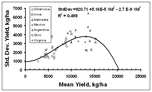
Figure 1. Average corn grain yield plotted against the coefficient of variation from by-plant yield over 46 transects in Argentina, Mexico, Iowa, Nebraska, Ohio, Virginia, and Oklahoma.
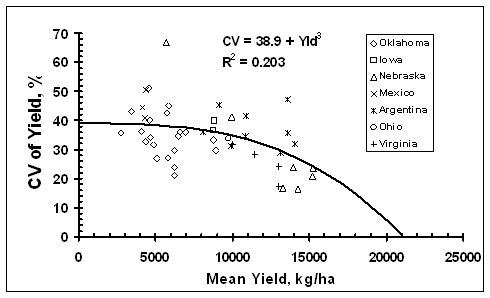
Figure 2. Average corn grain yield plotted against the by-plant yield range (max minus min) in 46 transects ranging from 10.5 to 30m in length, in Argentina, Mexico, Iowa, Nebraska, Ohio, Virginia, and Oklahoma.
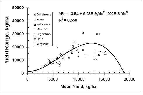
Figure 3. Average corn grain yield plotted against the standard deviation of by-plant yield over 46 transects in Argentina, Mexico, Iowa, Nebraska, Ohio, Virginia, and Oklahoma.
Figure 4. Average corn grain yields plotted by plant, every 2 plants, every 3 plants and every 4 plants, using measured distances between plants, Ames, IA 2004.
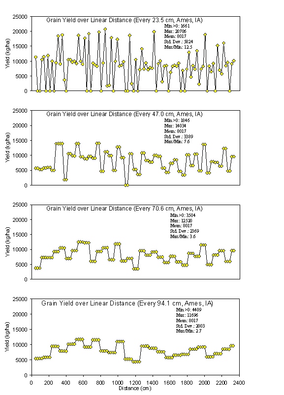
Figure 5. Average corn grain yields computed using fixed distances of 23.5, 47.0, 70.6, and 94.1 cm at Ames, IA 2004.
Yield =
-2348 + 18181(NDVI)
R2=0.49
Yield Mean: 8817
Standard Deviation: 1565
Figure 6. NDVI versus corn grain yield determined for every 4 plants using linear regression and associated 95% confidence intervals, east row, Ames IA, 2004
Figure 7. Effect of averaging plant yields over a specified distance along the row on the absoulute error incurred when using the average corn yield for estimating the by-plant yield. Yields were normalized by the average yield along the entire row.
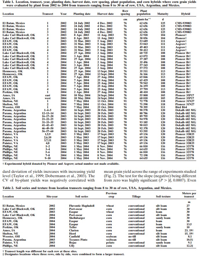
Table 4. Absolute value of the errors in estimating by-plant corn yield by averaging yield over a fixed distance along the row.
|
Distance (cm) |
Mean Error |
Maximum Error |
Minimum Error |
|
|
-----------------------------------Shelton, NE------------------------------------ |
||
|
15.0 |
5254 |
19562 |
0 |
|
30.0 |
4401 |
19562 |
65 |
|
45.1 |
3877 |
14961 |
13 |
|
60.1 |
3687 |
11249 |
12 |
|
75.1 |
3906 |
17271 |
24 |
|
90.1 |
3784 |
14170 |
3 |
|
1503 |
3569 |
1392 |
55 |
|
|
-------------------------------------Ames, IA------------------------------------- |
||
|
23.5 |
5497 |
22336 |
83 |
|
47 |
3588 |
17347 |
7 |
|
70.5 |
3101 |
16191 |
14 |
|
94 |
2937 |
15233 |
93 |
|
2352 |
2798 |
13519 |
7 |
|
|
------------------------------------EFAW, OK------------------------------------ |
||
|
20.1 |
3283 |
14634 |
0 |
|
40.1 |
2538 |
8962 |
56 |
|
60.2 |
2166 |
8227 |
76 |
|
80.2 |
2023 |
9207 |
15 |
|
100.3 |
2280 |
10030 |
15 |
|
2989 |
2473 |
10569 |
10 |
Agronomy Journal, 91:357-363